
Flight Analysis
1. This project only uses two years (2004 and 2005) out of all the years available in the dataset (1987 - 2008) due to memory and performance constraints. I will be redoing this analysis for the entire dataset soon using big data tools and updating it here.
2. Few of the reference links have also shut down or moved away from their domain so the references used will also be updated soon.
3. The explanations presented here and in the actual report may differ due to code changes done recently which are more efficient and calculate correctly.
Stay tuned!
Project Overview
This project explores flight data analysis and prediction patterns.
The main goals were:
- Analyze flight delay patterns and identify key factors
- Visualize air traffic trends and seasonal patterns
- Predict flight delays using machine learning models
The analysis is based on commercial flight data and combines statistical analysis and machine learning to obtain meaningful insights.
This project was done for University of London’s third year course ‘Programming for Data Science’ during my BSc. Economics degree. The full coursework question set can be found here ST2195_Coursework (PDF).
The questions are:
- When is the
- best time of day to fly to minimise delays?
- day of the week to fly to minimise delays?
- time of year to fly to minimise delays?
- Do older planes suffer more delays?
- How does the number of people flying between different locations change over time?
- Can you detect cascading failures as delays in one airport create delays in others?
- Use the available variables to construct a model that predicts delays.
Introduction
Airline travel is an immensely popular mode of transportation, with billions of people taking it every year [1]. In 2019, there were approximately 38.3 million flights worldwide, and while the COVID-19 pandemic caused a significant dip in air travel, the numbers are expected to rebound [1]. Despite increased efficiency since the start of flight travel, flight delays remain a persistent issue for travellers. Through data exploration and modelling, this study aims to analyse trends in flight delays, connections, and other factors, providing insight into how flight data evolves over time.
Data
The data is from the Data Expo 2009: Airline on time data found in the Harvard Dataverse [2]. The data has 29 variables detailing each flight. When reading the data for both Python and R, the files for the code should be in the data folder or the working directory must be set to where the data is located.
Data pre-processing
To start with, for the purposes of answering the specific questions within this report, most of the columns are not needed. Hence, only 13 variables will be used in the main data set that will be used for analysis. These variables and their descriptions are listed below (Table 1).
| # | Variable | Description (as stated / inferred) | Notes / Rationale |
|---|---|---|---|
| 1 | Year | 1987 – 2008 (only 2004 and 2005 used) | Core temporal key |
| 2 | Month | 1 – 12 | Seasonality |
| 3 | DayOfWeek | 1 = Mon to 7 = Sun | Day of week key |
| 4 | DepTime | Actual departure time (local, hhmm) | Delay calc |
| 5 | CRSDepTime | Scheduled departure time (local, hhmm) | Baseline schedule |
| 6 | ArrTime | Actual arrival time (local, hhmm) | Delay calc |
| 7 | CRSArrTime | Scheduled arrival time (local, hhmm) | Baseline schedule |
| 8 | TailNum | Plane tail number | Join to plane data |
| 9 | ArrDelay | Arrival delay, in minutes | Target component |
| 10 | DepDelay | Departure delay, in minutes | Target component |
| 11 | Origin | Origin airport code | Network effects |
| 12 | Dest | Destination airport code | Network effects |
| 13 | Year of manufacture | The year the plane was manufactured (from plane-data file) | Age analysis |
Table 1: Selected variables
The reason for this selection is because these variables were the only ones determined to be crucial in answering the questions posed. We can also see that it is quite a large dataset since it is reading 3.5 gigabytes even when only 12 (actually 13 including plane manufacture year) variables were selected, so determining the important variables and selecting only those helps with reducing memory errors. The last variable, year of manufacture, is from the plane-data file.
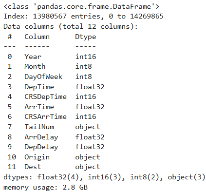
Table 2: Data information
The main dataset is first checked for NA/missing values. There are missing values in the variables DepTime, ArrTime, ArrDelay, and DepDelay. We can check how many NA values there are and see the percentage of them compared to the total amount of data. As a rule of thumb, dropping NA values that are less than 5% of the respective observations is acceptable [3]. As we can see, the variables that have NA values have them for less than 5% of their observations and hence, the NA values will be dropped.
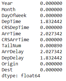
Table 2: NA percentage values
Now that the data is set, we can start to do analysis on the data.
Data Processing, Exploration and Modelling
When is the best time of day, day of the week, and time of year to fly to minimise delays?
The best time of the day
For Question 1 (best time of the day), to determine what is the best time of the day to fly, the variables CRSDepTime and CRSArrTime were selected. This is due to the fact that departure and arrival delays start at the scheduled departure and arrival timings. This would show the delays that are expected at a said scheduled time.
For example, if the scheduled departure time is 06 hours (6 AM) and the mean departure delay is found out to be one hour then the observation is that there is an expected mean departure delay of an hour after 6 AM. If the actual departure time was taken, this would be inverse in interpretation since the actual departure time would already consider the delay. If the actual departure time is 07 hours (7 AM) and the mean departure delay is the same, then the delay ended at 7 AM. Hence, the variables CRSDepTime and CRSArrTime were selected.
As shown in the hourly delay chart, the lowest mean arrival delay occurs at 6:00 and 7:00. The lowest mean departure delay is at 6:00, with a similarly low value at 7:00. The highest average delays for both arrival and departure are in the evening, especially between 17:00 and 21:00 (5 PM to 9 PM). Arrival delay spikes at 4:00, but this is not seen for departure delay. Delays drop after midnight, with arrival delays even turning negative at 6:00.
Figure 1: Interactive hourly mean delay
Thus, the best time to fly is early morning (6:00–7:00). To avoid delays, avoid evenings (17:00–21:00) and the early morning hour of 4:00.
The best day of the week
Next, we have the day of the week. First, the weekly data frame is created by extracting the variables DayOfWeek, ArrDelay, and DepDelay. This allows us to focus on just those variables for this part of the question and makes it easier to handle the data as well. The same goes for the monthly data frame where only Month, ArrDelay, and DepDelay were used. For both weekly and monthly analysis, total delay (the sum of arrival and departure delay) was calculated due to the fact that on a timeframe like a week or as large as a month, looking at arrival and departure delay separately seems excessive. On such a timescale, there will be very nuanced changes between the two types of delays especially on a monthly timescale and hence total delay was taken for both weekly and monthly analysis.
The weekly delay chart shows that Saturday has the lowest average delays, making it the best day to fly. Tuesday also has low delays. The highest average delays occur on Thursday and Friday. To minimize delays, fly on Saturdays or Tuesdays, and avoid Thursdays and Fridays.
Figure 2: Weekly mean delay
To minimize delays, fly on Saturdays or Tuesdays, and avoid Thursdays and Fridays.
The best time of the year (month)
According to the monthly delay chart, September has the lowest average delays, followed by April. The highest delays are in July, with December and June also showing elevated delay averages. These peaks correspond to summer and winter break periods. January and August have moderately high delays, likely due to seasonal effects.
Figure 3: Monthly mean delay
Do older planes suffer more delays?
For Question 2, the plane-data dataset was used. The NA values were checked and removed. The variable TailNum was used which then allowed for the year of manufacture to be extracted.
There are two regression lines in each plot. This is done due to the sampling difference mentioned in the data pre-processing. It is helpful to split the data and plot them in two sections within the same plot.
The regression plots split the data by year of manufacture (pre-1980 and post-1980) to account for sampling differences. Pre-1980, average delays increase with year, and the data is more scattered with a wider confidence interval. Post-1980, average delays show a slight downward trend and the data is less scattered. This suggests that, for newer aircraft, delays have decreased over time, while older planes pre-1980 experienced increasing delays. Sampling limitations for pre-1980 mean conclusions should be focused on the post-1980 data.
Figure 9: Regression plot of total delay against year of manufacture (Python)
How does the number of people (number of flights) flying between different locations change over time?
For Question 3, the data was split in two: pre-1980 year of manufacture and post-1980 year of manufacture. This is due to the sampling variations between the two periods. There are about 8 million observations in post-1980 compared to the 500,000 in pre-1980. Hence, it wouldn’t give an accurate representation if the two were not separated.
In both visualizations, we can see that there is quite a lot of change for most of the connections. The largest change is between DTW - TYS (Detroit, Michigan – Knoxville, Tennessee) where more than 90% of total flights were in 2004 which dipped to less than 5% of total flights in 2005. The second largest change is between LAS – PVD (Las Vegas, Nevada – Warwick, Rhode Island) where it had a little over 10% of total flights in 2004 which then increased to more than 80%.
DTW – SBN (Detroit, Michigan – South Bend, Indiana) and LGA – STT (Queens, New York – St. Thomas, US Virgin Islands) have about the same amount of change, percentage wise. Both had just below 40% in 2004 which increased to more than 60% in 2005. AKN – DLG (King Salmon, Alaska – Dillingham, Alaska) had the opposite change with 60% in 2004 dropping to 40% in 2005.
Figure 7: Top 5 connections by total flights (Python)
The R visualization is quite interesting, almost resembling a step graph. The largest change is, of course, between MSY – SLC (New Orleans, Louisiana – Salt Lake, Utah) where the percentage change is 100% which means that the flights in 2005 are double of those in 2004. The second largest is between GSO – TPA (Greensboro, North Carolina – Port Alsworth, Alaska) where there was an increase from 25% to 75% of total flights. There is a similar increase between GRB – MQT (Green Bay, Wisconsin – Gwinn, Michigan) where it increased from about 30% to 70% from 2004 to 2005. The connection between AKN – ANC (King Salmon, Alaska – Anchorage, Alaska) had almost no change at all with the percentage increasing from just below 50% to just a little over 50% from 2004 to 2005. A similar change is noted in BDL – IAH (Windsor Locks, Connecticut – Houston, Texas) with the increase being from about 45% to 55%.
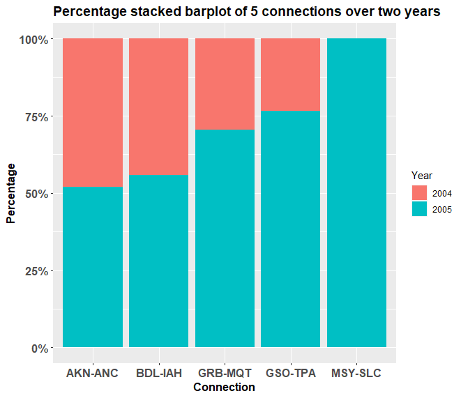
Figure 8: Top 5 connections by total flights (R)
Can you detect cascading failures as delays in one airport create delays in others?
For Question 4, two different data subsets were taken for Python and R. For Python, the top 5 connections, in ascending order, with total flights between 100 and 500 were analysed while for R, the top 5 connections, in ascending order, with total flights between 1000 and 2500 were analysed. This was done due to the fact that at higher levels of total flights, there is very little change since the total flights number is so large. Hence, to find a greater change between 2004 and 2005, the data was filtered and analysed.
Figure 13: Triangle correlation heatmap of top 5 airports (Python)
It is possible to detect cascading failures as delays propagate between airports. The correlation matrix shows how delay patterns are related across the five busiest hubs (ATL, DFW, EWR, ORD, PHL). Unlike perfect or very strong positive correlations, here we see a mix of weak positive, weak negative, and moderate correlations, which paints a more nuanced picture.
Negative correlations
ATL and EWR have a correlation of –0.54, the strongest negative relationship in the matrix. This suggests that when delays at ATL increase, delays at EWR tend to decrease, and vice versa.
ATL and ORD (–0.45) as well as ATL and DFW (–0.26) show moderately negative associations, implying that delays at Atlanta are often out of phase with those at Chicago and Dallas/Fort Worth.
EWR and ORD (–0.32) and EWR and PHL (–0.30) are also negatively correlated, suggesting that delays at Newark may relieve or counteract delays at these airports.
Positive correlations
DFW and EWR (0.31) show the highest positive relationship in the dataset, though it is still moderate. This could indicate some degree of shared delay propagation.
DFW and PHL (0.13) and DFW and ORD (0.08) are weakly positive, suggesting limited or inconsistent delay transmission.
Near-zero correlations
- ATL and PHL (–0.13) and ORD and PHL (–0.13) are very close to zero, indicating almost no systematic relationship in their delay patterns.
Overall, the lack of strong positive correlations means there is little evidence in this dataset of clear cascading failures like those seen in other analyses. Instead, the data suggests that delays may not consistently spread between these hubs, and in some cases, airports appear to move in opposite directions (negative correlations).
Use the available variables to construct a model that predicts delays
For Question 5, the variables that immediately impact arrival and departure delay were taken. These are CRSDepTime, CRSArrTime, DepTime, ArrTime, Origin, and Dest. Total delay was calculated, and the 6 variables were used to model total delay. The sample size taken for both Python and R is 200,000. A large sample size results in greater accuracy within the model. For R, the variables Origin and Dest had to be dropped due to the “Factor has new levels” error that occurs from taking samples. Unfortunately, this results in lower accuracy but the error could not be solved. The only solution found was to take the entire dataset but this would be impossible due to the fact that the data has about 7 million rows. This will result in numerous memory errors and session aborts from R. Hence, the variables were dropped. The models used are logistic regression and gradient boosting in Python and linear regression, ridge regression, lasso regression, and random forests in R.
The train-test split is 80-20. A large sample was used in order to improve accuracy. We can see that we have an AUC score of 0.89 for the gradient boosting while the logistic regression has an AUC of 0.71. An AUC score tells us how well a model can predict classes correctly [4][5][6]. An AUC score of 0.71 means that the logistic regression model can distinguish and predict 71% of the classes correctly. This is already a good score. Gradient boosting has a score 0.89 which means that it can predict 89% of the classes correctly. This is a high score and is close to being very high since it is just 1% below 90%. We can improve on the model by adding more variables that contribute to the delay [4]. We can also change the train-test ratio and see if it can improve the model.
Figure 15: Machine learning model (Python)
On the left is the graph visualizing the various mean squared error (MSE) values for the regression models. The values for each model are given in the table below. As we can see, the MSE values vary quite a bit. The random forest model has the highest MSE with the most range as well. Its mean MSE value is 26.6. The second highest is the ridge regression without any tuning. The third highest is the lasso regression without any tuning. The lowest is the linear regression. A MSE value of zero would imply a perfect model [7]. We cannot conclude this with the linear regression as such a small value when variables like Origin and Dest were dropped. It also threw a warning message that the “prediction from a rank deficient fit may be misleading”. This means that the test data did not work well with the regression [8]. The ridge and lasso regressions without tuning are more believable but these are without tuning. Their penalty terms, also called lambdas, have not been calculated when benchmarking [9]. We can (see) with the penalty terms that their MSE values fall drastically. We can improve upon the model by including more variables, especially origin and destination.
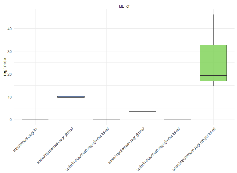
Figure 16: MSE values of regression models (R)
Conclusions
Overall, we were able to analyse when delays occur, changes in flight connections, cascading delays etc. There can be much more flight analysis done with this data. The entirety of the code, both in Python and R, took around 30 minutes to run and execute which is quite fast considering the samples taken in the machine learning models.
References
- The World of Air Transport in 2019. (n.d.). Retrieved March 25, 2023. Available at: Link
- Harvard Dataverse. (2008, October 6). Data Expo 2009: Airline On Time Data. Retrieved February 27, 2023. Available at: Link
- Mears, K., Montelpare, W. J., Read, E., McComber, T., Mahar, A., & Ritchie, K. (n.d.). Working with missing data. Retrieved April 3, 2023. Available at: Link
- Allwright, S. (2022, August 23). What is a good AUC score? Retrieved April 2, 2023. Available at: Link
- Google Developers. Classification: ROC curve and AUC. Retrieved April 1, 2023. Available at: Link
- Bhandari, A. (2023, March 28). Guide to AUC ROC curve in machine learning. Retrieved March 25, 2023. Available at: Link
- Allwright, S. (2022, December 6). What is a good MSE value? Retrieved April 2, 2023. Available at: Link
- ProgrammingR. Fix R warning: Prediction from a rank-deficient fit may be misleading. Retrieved April 1, 2023. Available at: Link
- Andrea Perlato. Ridge and lasso regression. Retrieved April 2, 2023. Available at: Link
📂 Project Files
🔗 Repository
Source code and materials are available on GitHub:
👉 Flight Analysis Repository