
Price Discrimination Strategies of Air India and Vistara on the Delhi-Mumbai Route
Project Overview
This project explores the concept and real-world application of price discrimination in economics.
The main goals were:
- Illustrate different types of price discrimination (first, second, and third degree) with examples
- Analyze how firms segment markets and set prices for different consumer groups
- Discuss fairness, ethical, and legal considerations in price discrimination practices
The project uses real-world data and economic models to demonstrate pricing strategies and their implications.
Introduction
The airplane has been a popular mode of transport globally for close to 80 years now. It has become a popular mode of transport domestically within India as well as Indians are able to now afford airplane tickets alongside the emergence of Indian airline companies that are either full-service airlines or low-cost airlines. It is no doubt that the Indian airline market will grow even more in the coming years. According to Gupta (2024), the Indian domestic airline market is already the 3rd largest in the world. As for the airlines that serve the domestic market, according to Anand (2023), the market share was broken up into IndiGo (63.3%), Air India (9.8%), Vistara (9.8%), AirAsia (7.1%), SpiceJet (4.4%), and Akasa Air (4.2%).
The main thing that every consumer is dealing with is the price of a ticket when travelling by air. However, anyone who travels regularly or even checks airplane ticket prices will notice that the prices change a lot. They change due to holiday seasons, peak timings either during the week or the day, how long the flight is, whether there are stopovers, the ticket class etc. There are a lot of factors that can influence the price of a seat. It is important to understand how airlines price the tickets and how the prices change as the factors themselves change. This is called price discrimination which is practiced heavily in the airline industry. It is also called dynamic pricing as the prices depend on time as well. We will look at the theory of price discrimination, review the existing literature regarding price discrimination in the airline industry, and then perform data analysis.
Theory of Price Discrimination
Price discrimination is essentially when firms charge different prices to different consumers for the same good. This is the case within the airline industry as firms are selling airline tickets for different prices depending on a lot of factors. There are various ways this can be done but price discrimination has been broken down into three categories: first, second, and third.
First degree price discrimination, also called perfect price discrimination, is when the firm is able to charge a different price for each and every consumer. The price charged by the firm here will be the consumer’s maximum willingness to pay. This eliminates the consumer surplus of consumers and leaves them indifferent between consuming a good or not (Snyder, 2007). In reality, this is not possible since firms cannot know the maximum willingness to pay for every consumer.
Second degree price discrimination is when the price depends on the quantity or quality bought. Firms will charge different prices for different quantities or quality of the same good (Pindyck, 2018). An example is the pricing for a plane seat that is sold in different types like economy, business etc.
Third degree price discrimination is when the firms can divide consumers into groups and charge different prices to each group based on the observable group characteristics (Pindyck, 2018). This also happens in the airline industry where airline companies price consumers based on the booking time, number of stops etc.
Third degree price discrimination is the most practiced price discrimination within the airline industry. Airlines focus on segregating customers based on timings, duration etc. Additionally, second degree price discrimination is also followed whereby airlines segregate flyers based on leisure or business flyers and accordingly accommodate economy and business class.
Literature Review
Before starting the discussion on data and data analysis, a brief literature review will be conducted.
Dutta and Santra (2015) analyze the price movements and discrimination in the Indian airline market. The main objectives were to analyze the trend in prices as departure days draw closer, the effect of different days of the week on prices etc. The paper used one month data for 69 airlines across India and built regression models based on various variables such as day of the week, route, days before departure etc. The paper found that prices increased in the lead up to the departure date and also featured jumps in prices which has been attributed to the block pricing strategy. The block pricing strategy is akin to the second degree price discrimination. It also found that prices were much higher on weekends as compared to weekdays. The routes have their own attributes due to differing demands, operational costs etc. along these routes. As such, the prices are mainly set based on these route attributes, the days before departure, and the day of the departure itself.
Bankole (2024) analyzes the strategies of price discrimination within the airline industry. The paper found that airlines use prices tailored to groups of flyers and different advance booking windows.
We can see that airlines mainly set their strategies based on days before departure, duration, time of departure etc which is characteristic of third degree price discrimination. The airlines also use second degree price discrimination based on the seat class. As such, airlines use both strategies in order to set differing prices.
Data and Research Question
The data for price discrimination analysis was taken from Kaggle, which was scraped from Ease My Trip, which contained prices from six different airline companies with six different cities for departures and arrivals. The airline companies were Air India, Air Asia, Go First, Indigo, Spice Jet, and Vistara. The departure and arrival cities were Bangalore, Chennai, Delhi, Hyderabad, Kolkata, and Mumbai. The data is from February 11 to March 31, 2022.
To reduce the complexity of the analysis and focus on price discrimination, we have chosen Air India and Vistara as the airline companies and the Delhi-Mumbai route (and vice versa) for analysis. The two companies were chosen as they provide business and economy class seats on the Delhi-Mumbai route. The other four airline companies only provide economy flights. As such, to keep the analysis consistent, we chose the two companies that provided both ticket classes. Air India and Vistara also account for 70% of the flights along this route. As such, it was clear to choose the two companies for analysis. Figure 1 shows a snippet of the sample data.
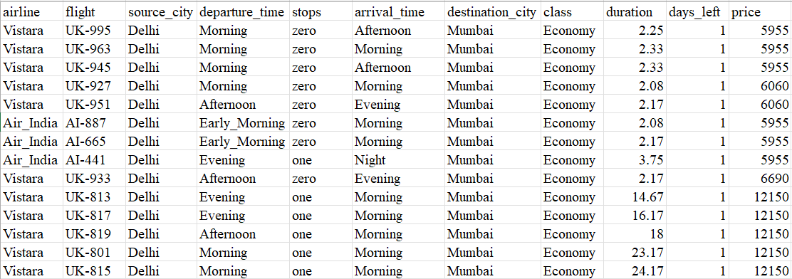
Figure 1: A snapshot of the data used
Source: Dataset taken from Kaggle, data was scraped from Ease My Trip
Hence, the research question is “How do the factors influencing airlines’ pricing strategies affect price discrimination on the Delhi-Mumbai route for Air India and Vistara?”. The focus point is to see how class, number of stops, departure time, arrival time, duration, and days left affect the ticket price.
Data Analysis
We can first start with observing the trends of the average prices of both classes plotted against the days remaining before the flight. Figure 2 shows the average price of economy class plotted against the days remaining before the departure.
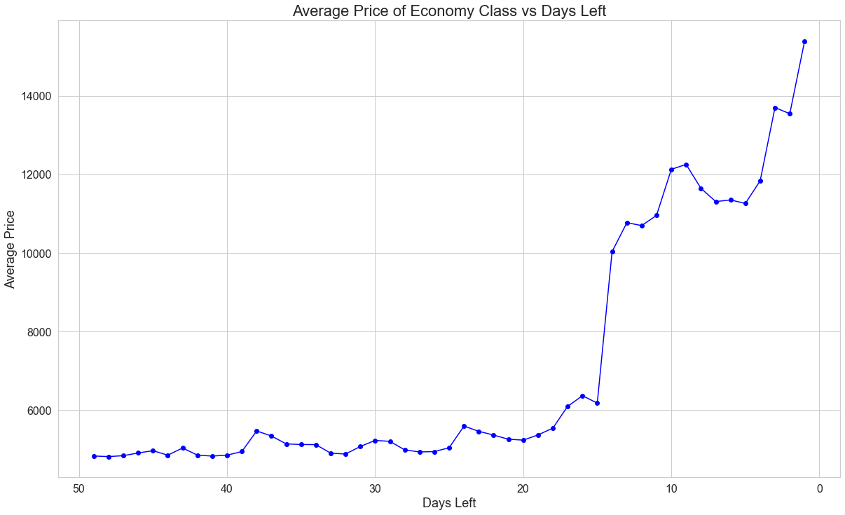
Figure 2: Average price of an economy class ticket as departure day draws closer
Source: Coded in Python by authors
We can see that the average price has stayed relatively low, between ₹2,500 to almost ₹6,000, after which there is a sharp increase around 15 days before the flight. The average price jumps from ₹6,000 to ₹10,000 within one day. This is a massive increase in the average price. Ultimately, the average price reaches somewhere around ₹16,000 just one day before the flight. The trajectory of the average price is understandable as many people book their flight tickets around two weeks, i.e. 14 days, before the flight. The average price also keeps increasing as the seats of the flight get booked and so supply of the seats shrink while demand increases. As such, due to demand and supply dynamics as well as airline pricing strategies based on remaining capacity, the price will rise.
We can also look at the average prices within the business class. Figure 3 shows the average price of business against days remaining to the flight. We can see that the average price hikes just 5 days before the flight. This is expected as there are fewer number of people that choose business class and the demand for it will only heighten within the last one week or so. We can see that the average price remained relatively steady around ₹43,000 to ₹45,000 but then jumped dramatically to ₹52,000 within the span of 3 – 4 days.
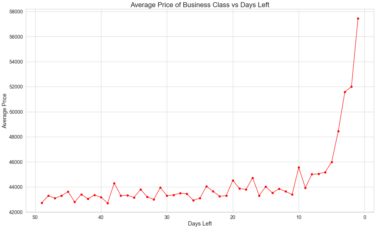
Figure 3: Average price of a business class ticket as departure day draws closer
Source: Coded in Python by authors
We can also check how the price changes for both the classes based on the duration of the flight. Figure 4 shows the scatterplot and average price of economy class with respect to the duration of the flight.
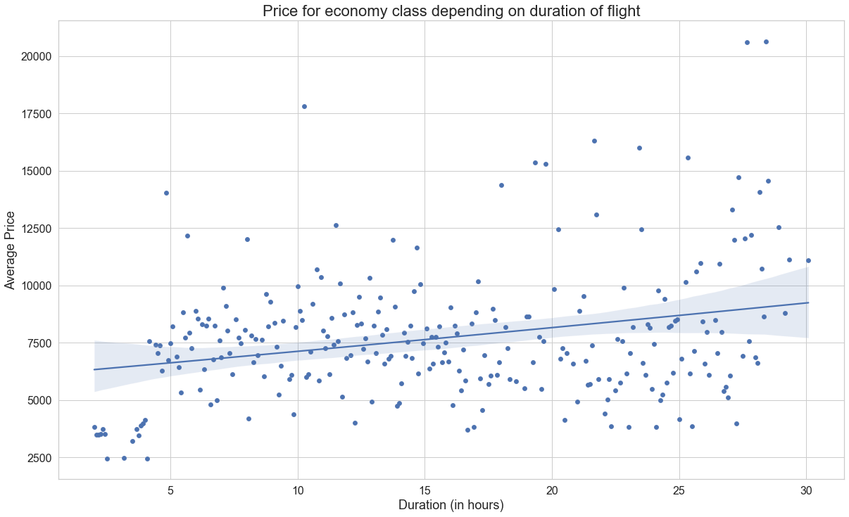
Figure 4: Price of economy class depending on flight duration Source: Coded in Python by authors
We can see that there is quite the scatter of prices and that the prices slightly increase as the duration of the flight increases. This is represented by the upward sloping trendline for average prices. This is expected as higher duration of a flight will represent higher fuel and operational costs. The data also contains stops which is counted in the duration. As such, the higher duration flights most likely have stops and as such will have higher costs.
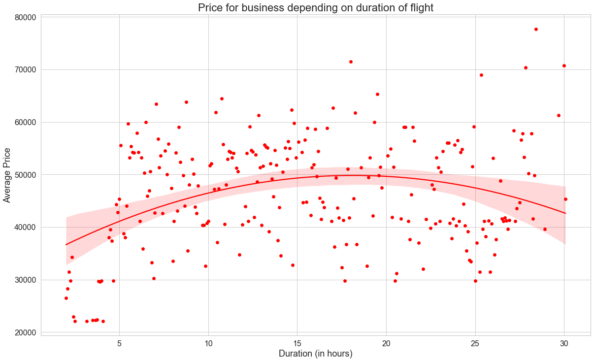
Figure 5: Price for business class depending on flight duration
Source: Coded in Python by authors
Figure 5 shows the scatterplot and average price of business class with respect to the duration of the flight. The trendline for business class is much more curved. The points are also much more scattered compared to economy class. However, we can still see the increase in prices as the duration of the flight increases very distinctly. It starts around ₹35,000 and then increases to ₹50,000 at its highest point and then dropping down according to the trendline.
Price Ratio
We can also check the ratio of the average prices 1 day before departure and 49 days before departure. 49 days is the maximum number of days before departure given in the dataset. This ratio will allow us to check how much more expensive the flight is 1 day before departure compared to 49 days before departure. Average values will be calculated for both 1 day before departure and 49 days before departure. This ratio will be calculated for both economy and business class.
For economy class, the values are:
\[\frac{P_{(-1)}}{P_{(-49)}} = \frac{15,397.744}{4,834.62} = 3.18\]This means that the flight ticket is 3.18 times more expensive when comparing the price 49 days before departure to just 1 day before departure.
For business class, the values are:
\[\frac{P_{(-1)}}{P_{(-49)}} = \frac{57,457.83}{42,736.48} = 1.34\]The price ratio is much lower for business class when compared with economy class. The price for business class will only increase by 1.34 when comparing the price 49 days before departure to just 1 day before departure. This indicates that the price of a business class ticket does not change as much when the departure date is approaching as compared to economy class.
In general, it is observed that prices are lower for connecting flights than direct flights. Figure 6 shows the average prices by number of stops. We can see that the average prices are higher when there is a stop compared to when there is not one. This is expected as stops will be associated with higher costs as it may be perceived as inconvenient. However, it must be noted that this is not always the case. Sometimes, connecting flights are priced lower by the airline in order to attract customers since it takes longer and is less convenient. According to the data, connecting flights have been priced higher.
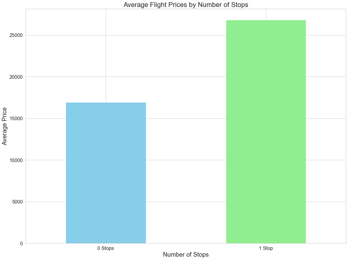
Figure 6: Average prices of flight based on the number of stops
Source: Coded in Python by authors
Regression Analysis
We will also run a regression analysis in order to estimate the coefficients of variables and interpret their impacts on ticket price. The regression model will contain ticket price as the dependent variable and departure time, arrival time, number of stops, class, duration, and days left till departure as the independent variables. The regression model can be written as:
\[\begin{align} \text{Price} = \ &\beta_0 + \beta_1 \cdot \text{class} + \beta_2 \cdot \text{departure time} + \beta_3 \cdot \text{arrival time} \\ &+ \beta_4 \cdot \text{number of stops} + \beta_5 \cdot \text{duration} + \beta_6 \cdot \text{days left} + \varepsilon \end{align}\]Class, departure time, and arrival time are all categorical variables. As such, dummy variables must be created so that regression can be performed. Class is split into economy and business so the dummy variable will be defined as:
\[D_c = \begin{cases} 0 & \text{if economy} \\ 1 & \text{if business} \end{cases}\]Departure time is split into five categories: early morning, morning, afternoon, evening, and night. Arrival time is split into six categories: early morning, morning, afternoon, evening, night, and late night. Since dummy variables can only take binary values, we have made five dummy variables for departure time and six for arrival time. Afternoon is taken as reference for both departure and arrival times.
The dummy variables for departure times are:
\[\begin{align} D_{D-EM} &= \begin{cases} 1 & \text{if departure is in early morning} \\ 0 & \text{otherwise} \end{cases}\\ D_{D-M} &= \begin{cases} 1 & \text{if departure is in morning} \\ 0 & \text{otherwise} \end{cases}\\ D_{D-E} &= \begin{cases} 1 & \text{if departure is in evening} \\ 0 & \text{otherwise} \end{cases}\\ D_{D-N} &= \begin{cases} 1 & \text{if departure is at night} \\ 0 & \text{otherwise} \end{cases} \end{align}\]The dummy variables for arrival times are:
\[\begin{align} D_{A-EM} &= \begin{cases} 1 & \text{if arrival is in early morning} \\ 0 & \text{otherwise} \end{cases}\\ D_{A-M} &= \begin{cases} 1 & \text{if arrival is in morning} \\ 0 & \text{otherwise} \end{cases}\\ D_{A-E} &= \begin{cases} 1 & \text{if arrival is in evening} \\ 0 & \text{otherwise} \end{cases}\\ D_{A-N} &= \begin{cases} 1 & \text{if arrival is at night} \\ 0 & \text{otherwise} \end{cases}\\ D_{A-LN} &= \begin{cases} 1 & \text{if arrival is at late night} \\ 0 & \text{otherwise} \end{cases} \end{align}\]Hence, the regression model in its entirety is:
\[\begin{align} \text{Price} = \ &\beta_0 + \beta_1 \cdot D_c + \beta_2 \cdot D_{D-EM} + \beta_3 \cdot D_{D-E} + \beta_4 \cdot D_{D-M} + \beta_5 \cdot D_{D-N} \\ &+ \beta_6 \cdot D_{A-EM} + \beta_7 \cdot D_{A-E} + \beta_8 \cdot D_{A-LN} + \beta_9 \cdot D_{A-M} + \beta_{10} \cdot D_{A-N} \\ &+ \beta_{11} \cdot \text{stops} + \beta_{12} \cdot \text{duration} + \beta_{13} \cdot \text{days left} + \varepsilon \end{align}\]We have omitted afternoon since it is the reference category in order to avoid multicollinearity. We can now conduct regression on this in Python. The regression results are as shown below in Figure 7.
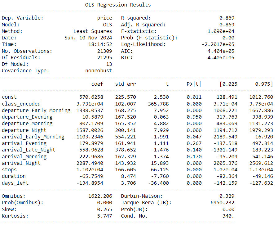
Figure 7: Regression results
Source: Coded in Python by authors
Interpretation of Results
We can see that \(\beta_0 = 570.63\) which means this is the baseline price when all variables are zero. However, this serves no purpose with regards to interpretation as a flight with zero duration or no departure and arrival times does not exist.
The coefficient of class is \(\beta_1 = 37,310\). This indicates that changing from economy to business adds ₹37,310 to the ticket price. \(\beta_1\) is also statistically significant since its p-value is less than 0.05.
The coefficient of early morning departure is \(\beta_2 = 1,338\). This indicates that choosing early morning departure adds ₹1,338 to the ticket price. \(\beta_2\) is also statistically significant. This indicates that early morning departure does have a significant impact on price.
The coefficient of evening departure is \(\beta_3 = 10.58\). However, this value is not statistically significant since its p-value is 0.950 which is greater than 0.05. This suggests that evening departures have no significant impact on price.
The coefficient of morning departure is \(\beta_4 = 807\). This implies that morning departure adds ₹807 to the ticket price. \(\beta_4\) is statistically significant as well.
The coefficient of night departure is \(\beta_5 = 1,587\). This shows that choosing night departure adds ₹1,587 to the ticket price. \(\beta_5\) is statistically significant as well. Of all the departure timings, early morning and night departures add the most to the ticket price.
As for arrival timings, evening (\(\beta_7\)), late night (\(\beta_8\)), and morning (\(\beta_9\)) coefficients are all statistically insignificant as their p-values are higher than 0.05 at 0.267, 0.140, and 0.170 respectively.
The coefficient for early morning arrival is \(\beta_6 = -1,103.23\). This indicates that choosing early morning arrival reduces the ticket price by ₹1,103. Meanwhile, the coefficient for night arrival is \(\beta_{10} = 2,287.49\). This means that night arrival will increase price by ₹2,287.5. Both coefficients are statistically significant since their p-values are less than 0.05.
The coefficient for stops is \(\beta_{11} = 11,020\). The interpretation here is that each additional stop adds ₹11,020 to the ticket price. This is also statistically significant. The reason for such an increase in price may be due to operational costs or complexities regarding landing and itinerary.
The coefficient for duration is \(\beta_{12} = -65.75\). This indicates that each additional hour of flight will reduce the ticket price by ₹65.75. This is statistically significant but the effect is relatively small. One reason for this may be to attract demand on longer flights.
The coefficient for days left until departure is \(\beta_{13} = -134.9\). This indicates that each additional day before departure, the ticket price will decrease by about ₹134.9. This is statistically significant and also consistent with the previous analysis as shown in Figures 2 and 3 where the prices rise drastically just 2 weeks before departure for economy class and 1 week before departure for business class.
We also evaluate the model as a whole. The \(R^2\) value is 0.869 which means that 86.9% of the variability in prices is being explained by the model. The adjusted \(R^2\) value is also 0.869 which means that the explanatory power of the model is not affected by the number of predictors. Hence, the model explains the variation in price well.
The regression model with the coefficient values that are statistically significant is given by:
\[\begin{align} \text{Price} = \ &570.63 + 37,310 \cdot D_c + 1,338 \cdot D_{D-EM} + 807.17 \cdot D_{D-M} + 1,587 \cdot D_{D-N} \\ &- 1,103.23 \cdot D_{A-EM} + 2,287.49 \cdot D_{A-N} + 11,020 \cdot \text{stops} \\ &- 65.75 \cdot \text{duration} - 134.895 \cdot \text{days left} \end{align}\]Example Calculation
An example can be taken where the chosen attributes are economy class, night departure, early morning arrival, one stop, 6 hours of flight, and booked 7 days before departure. The calculation of price is then:
\[\begin{align} \text{Price} = \ &570.63 + 1,587 \times 1 - 1,103.23 \times 1 + 11,020 \times 1 \\ &- 65.75 \times 6 - 134.895 \times 7 \\ = \ &10,735.64 \end{align}\]The price is then ₹10,735.64. We can use the same attributes but now for business class. The price is then:
\[\begin{align} \text{Price} = \ &570.63 + 37,310 \times 1 + 1,587 \times 1 - 1,103.23 \times 1 + 11,020 \times 1 \\ &- 65.75 \times 6 - 134.895 \times 7 \\ = \ &48,045.64 \end{align}\]We can see that the price jumps by ₹37,310 which leads the total price to ₹48,045.64.
Limitations of the Analysis
There are plenty of limitations of the analysis that we have done. These are:
1. No Quantity Data
The data and the model has no input of quantity. Quantity is an important tool to analyze price discrimination. However, since there is no quantity data, it is not a full analysis of price discrimination. As of now, this analysis is only focusing on the factors that airlines use to set prices. With quantity data, it would be possible to analyze how different consumer demands are changing against prices.
2. Omitted Variables
The model has been built with the variables given in the data. However, it is possible that there are omitted variables. A possible omitted variable is the competition from other airlines on the same route. While Air India and Vistara account for 70% of the flights along this route, the 30% of flights by other airlines can still affect the prices that are set by Air India and Vistara. Omitted variables can lead to biased coefficients especially if the omitted variables are correlated with the variables used.
3. Stationary Coefficients
The coefficients are stationary since the model assumes that coefficients do not change with time. However, the coefficients can change with time. This is mainly due to external factors such as fuel costs, economic shocks etc. Due to this, the model may predict incorrectly for certain periods.
4. Assumption of Linear Relationship
The model assumes a linear relationship between the price and the independent variables. However, it is likely that independent variables may have nonlinear effects on price. This can oversimplify the results and interpretations.
Conclusion
In conclusion, the analysis examined how factors such as class, number of stops, departure and arrival times, flight duration, and days before departure influence ticket prices on the Delhi-Mumbai route for Air India and Vistara. The analysis showed a clear trend of price discrimination such as with varying prices between business and economy class tickets or the prices rising as departure dates get closer. There is clear second and third degree price discrimination being practiced.
The regression analysis supports these findings, with significant coefficients for class, stops, departure time, and days before departure. However, limitations such as the absence of quantity data and potential omitted variables like competition from other airlines on the same route suggest that the model could be improved. The model may also be oversimplified due to the assumption of linear relationships between price and the independent variables.
Overall, the analysis shows how Air India and Vistara use dynamic pricing strategies to maximize their revenue. Future research should explore how the quantity changes with price in various market segments, the impact of competition from other airlines, and how this differs across multiple routes.
References
- Anand, S. (2023). Indian Aviation Market Share Analysis
- Bankole, A. (2024). Price Discrimination Strategies in the Airline Industry
- Dutta, P., & Santra, S. (2015). Price Movements and Discrimination in the Indian Airline Market
- Gupta, R. (2024). Global Aviation Market Rankings
- Pindyck, R. S. (2018). Microeconomics. Pearson Education
- Snyder, C. (2007). Price Discrimination Theory and Applications
🔗 Repository
Source code and materials are available on GitHub:
👉 Price discrimination Repository