Project Overview

This project analyzes Brazil’s monetary policy using the Taylor Rule framework.
The main goals were:

• Apply the Taylor Rule to Brazil’s economic data to model interest rate decisions
• Compare actual central bank policies with Taylor Rule predictions
• Visualize the relationship between inflation, output gap, and policy rates over time

The study uses empirical data, economic modeling, and visualizations to assess how closely Brazil’s policy aligns with standard monetary guidelines.

Introduction

The debate on whether monetary policy should be based on intuition or a policy rule has been going on since the 19th century. After the Great Depression, policies came under great scrutiny. Monetarists like Milton Friedman opined that high inflation could have been curbed if the Federal Reserve had managed the money supply consistently.

The Taylor Rule, propounded by Stanford economist John Taylor, is an interest rate policy which was outlined in his 1993 paper titled “Discretion Versus Policy Rules in Practice.” The rule dictates how interest rate must be changed by the Central Bank to account for inflation and other economic conditions. In simple terms, the rule suggests that when inflation rises or growth (GDP) exceeds targets, the interest rate too must be increased. Contrarily, when inflation falls or growth falls below potential, the interest rate must be reduced.

The Taylor’s Rule considers both the difference between the actual and targeted inflation rates and the difference between the desired and actual output also known as the output gap. The rule reduces the Central Bank’s discretionary policies and suggests a standardized rule for interest rate changes.

The Basic Setup of the Taylor Rule

According to Taylor (1993), the Taylor Rule can be setup as:

Where:

• \(r\) is the federal funds rate
• \(p\) is the rate of inflation over the previous four quarters
• \(y\) is the percent deviation of real GDP from a target. That is, \(y = \frac{Y - Y^*}{Y^*} \times 100\) where \(Y\) is real GDP, and \(Y^*\) is trend real GDP.

The equation assumes the equilibrium federal funds rate of 2% above inflation, represented by the sum of \(p\) (inflation rate) and the 2 on the far right. 0.5 is a weighting factor, indicating the relative importance of inflation and the output gap.

From that equilibrium, the federal funds rate is assumed to move up or down by half the difference between actual and targeted inflation, with overshoots relative to the target increasing the rate and undershoots lowering it.

The other variable is the output gap or the difference between actual and targeted growth in real GDP. As with inflation, each percentage point of the output gap moves the expected federal funds rate by half a percentage point, with growth above target raising it and shortfalls lowering it. In simpler terms: The Taylor Rule suggests raising the Federal Funds Rate when inflation is above 2% or when the economy is operating above its potential (output gap is positive), and lowering the rate when inflation is below 2% or when the economy is operating below its potential (Hayes, 2023).

What does the Taylor Rule try to predict?

The Taylor Rule predicts that the Federal Reserve will raise the federal funds rate - which is the target interest rate it sets for banks to borrow and lend reserves overnight - by half a percentage point for each percentage point that inflation rises relative to its 2% target, or for each percentage point that GDP exceeds its potential. In doing so, the Fed would be engaging in a form of monetary tightening.

The Taylor’s rule also predicts that when inflation is at target and output is at potential that is, when the output gap is zero, the Central bank will set the real federal funds rate at 2% which according to Taylor was its historical average (Bernanke, 2015).

Relevance of Taylor Rule

John Taylor has been quite critical about the Federal Reserve’s policies. According to him, the Federal Reserve kept interest rates much lower than prescribed by the Taylor rule during 2003-2005. Some economists believe that the central bank was at least partly responsible for the housing crisis in 2007-2008. The interest rates were kept too low in the years following the dot-com bubble and leading up to the housing market crash in 2008. Had the central bank followed the Taylor rule, the interest rate would have been much higher. As a result, the bubble may have been smaller, as fewer people would have been incentivized to buy homes (Twomey, 2024).

This deviation was a major source of the housing bubble and other financial excesses. Taylor also asserts that the Federal Reserve’s monetary policy since the financial crisis has not been sufficiently rule-like. Had they been following the Taylor rule, it would have ended its policy of near-zero interest rates several years ago (Bernanke, 2015).

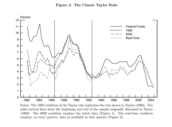
Figure 1: The Classic Taylor Rule from 1982 to 2002. Source: (Orphanides, 2003)

Country Selection

Since this research will focus upon a specific country to conduct analysis, we need to select and justify the selection of a country. There are many candidates such as the United States (US), the United Kingdom (UK), Japan, and the countries of the European Union just to name a few. However, we decided to choose Brazil as the country to do our analysis on.

Brazil is an excellent country to do Taylor Rule analysis on mainly due to:

1. The inflation-targeting regime set by the Central Bank of Brazil (BCB) in 1996. This determines how the BCB conducts open market operations and is the bank’s overnight rate, the SELIC rate. The SELIC rate is the BCB’s main instrument of monetary policy (BCB, n.d.).

2. In the past, Brazil has faced heavy inflation especially two periods of hyperinflation around 1990 and then around 1993. The Real plan of 1996 which also introduced the inflation-targeting regime and set up the monetary policy committee (COPOM) to monitor it. We can see that since then, inflation has been consistently kept low in comparison to the hyperinflation that was experienced.

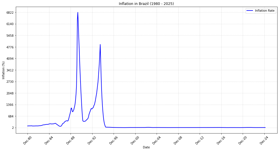
Figure 2: Inflation rate in Brazil (Source: Central Bank of Brazil)

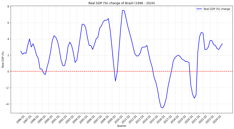
Figure 3: Real GDP Percent Change of Brazil (Source: System of Quarterly National Accounts - IBGE)

1. Brazil has gone through recessions which has tested the capabilities of policy responses. While COVID-19 was certainly one recession for the economy, the 2015-2016 recession was far more severe to the economy. This is shown by figure 3.

Historical Taylor Rule in Brazil

The Taylor’s rule has been considered by the Brazilian Central Bank in its macroeconomic policy making since their adoption of an inflation targeting regime in 1999. Since then, Brazil has gone through a remarkable process of stabilization followed by an economic boom from 2004. A crucial element in making the country more resilient to shocks like the 2008 financial crisis and the European debt crisis was their cautious and rule based monetary policy.

The BCB maintained the annual overnight interest rate (SELIC) higher than what a straightforward Taylor rule would have recommended for the first period, which ran from July to September 1999. Inflation was quite mild when the inflation targeting framework was introduced in July 1999, but it was predicted to increase. This was a stricter policy than what would have been implied by a straightforward Taylor rule. This was taken by the BCB out of concern about an increase.

The second phase, which spanned October 1999 to January-February 2000, had a sharp increase in inflation, which peaked in December 2000. BCB did not increase the SELIC, contrary to what a straightforward Taylor rule would have indicated. It is evident that even though inflation was greater than anticipated in the final quarter of 1999, this was thought to be temporary. Consequently, the real SELIC was maintained at a rate that was marginally lower than what our straightforward Taylor rule would have predicted.

February and March 2000 marked the beginning of the third period. During this time, inflation has stayed within the inflation target range and has been declining. The actual SELIC has stayed within the Taylor rule’s bands as a result of the decline in inflation (Mario I. Blejer, 2001).

Literature Review

Now that we have a basic understanding of how the Taylor’s Rule works, we delve into the empirical analysis of this rule and see what were the effects on the countries that adopted this rule and what changes were brought upon due to this:

We look at few research papers that give us an insight into the practical application and effect of Taylor’s Rule:

The Taylor Rule: A Benchmark for Monetary Policy? Brookings Institution (Bernanke, 2015)

The author sheds light on the main concept of Taylor’s Rule, its theoretical construct, origins, effect after application and practical implications of the same and emphasizes its role as acting as a guideline for monetary policy. Based on the theoretical concepts the author says that the rule is derived from the principles of optimal monetary policy which was derived with the aim of stabilizing inflation and output. The rule further provides a reliable and predictable guideline for central banks which helps reduce risks with discretionary policy decisions. Coming to the Empirical analysis of the same, we see through this paper that United States was empirically successful in using the Taylor’s Rule. This can be seen through the Federal Reserve’s Policy during the Great moderation period that was around (1980s-2007), the effect seen for the same was that the period saw low inflation and stable economic growth. For example, the Fed’s interest rate decisions during this period were well-explained by the rule, which helped anchor inflation expectations and stabilize output fluctuations which made it a popular source for assessing better monetary policy due to its simplicity and transparency.

Did The Taylor Rule Stabilize Inflation in Brazil? (De-Losso, 2008)

This paper tries to examine Taylor’s rule in the emerging markets of Brazil and investigate in its practical implication and understand the effects on the country by doing the same. The author Rodrigo De-Losso takes in account three different periods to analyse the effectiveness of Taylor’s Rule. The study mainly tries to analyse this by using a forward looking Taylor rule type reaction in order to have insights to analyse Brazilian monetary policy from 1980 onwards. The three periods that the author discusses in this paper is: First, the Megainflationary Era which was from the period of (1980 – 1994) where inflation had skyrocketed to nearly 500% per year to the response of which the policymakers reacted aggressively to inflation. The Second period, was the Real Plan Era which was from the period of (1994-1999). Here, the inflation had lowered down to roughly 8% per year which happened after the Real Plan was introduced. The third period, The Inflation Targeting Era (2000 onward) where Brazil utilised an explicit inflation – targeting framework. Now that we understand better what happened in these three periods, we now take a look at the effects the rule had. Before the Real plan had been implemented, the predictions that were given by the Taylor’s Rule were not consistent enough given the observed monetary instability. Though the interest rate response to inflation was high, inflation was still not controlled which suggested that inflation coefficient greater than one does not necessarily stabilize prices. After the real plan had been implemented we know through the Taylor rule that if the inflation coefficient was less than one stability could not be achieved. However, we see here that though inflation coefficient was less than one monetary stability was still achieved which also indicate that that stability in monetary policy can still be achieved even when the interest rate response is below one to one. Post 2000s the empirical results showed that although there was a loose monetary policy, the inflation still remained under control. This study challenged the conventional norms of the Taylor rule as it showed that not necessarily strong interest rate response would guarantee monetary stability and vice-versa. Another thing to note was that Brazil’s monetary authorities were forward looking in setting interest rates, rather than looking at past inflation.

The Central Bank of Brazil’s time-varying Taylor rule (Filipe Gropelli Carvalho, 2022)

The authors of this paper aimed to investigate how the Central Bank of Brazil (BCB) applied the Taylor rule across time and how monetary policy preferences evolved. Using a time-varying parameter (TVP) approach, they examined two characteristics: the Taylor rule inflation response coefficient and the BCB’s implicit inflation target. They were interested in observing if the BCB strictly followed the Taylor principle, or raised interest rates proportionally more than inflation, and also how it shifted its policy between different ranges of time. It was revealed that during the period from 2003 to 2011, the BCB pursued a hawkish policy stance, that is, the central bank was very keen about confronting inflation. During this period, the Taylor rule managed to maintain inflation as well as macroeconomic stability. From 2011, however, the BCB became dovish and was more concerned with economic growth than with inflation control. This reduced the inflation response coefficient considerably, which indicated that the central bank did not care so much about suppressing inflation, thereby resulting in more inflation volatility. By estimating the implicit inflation goal, the authors further observed that while the BCB tended to stay within official inflation target levels established by the National Monetary Council (CMN), there existed serious deviations, particularly between the periods 2011-2016. Based on their results, deviations from the Taylor rule have the capacity to weaken its effectiveness in handling inflation and expectations. Yet they also point out that even the rule remains a good guide to monetary policy, if only it is applied consistently and flexibly.

Estimating Monetary Policy Reaction Functions for Emerging Market Economies: The Case of Brazil (Sánchez-Fung, 2011)

The paper “Estimating Monetary Policy Reaction Functions for Emerging Market Economies: The Case of Brazil” by provides an example of how the Brazilian central bank applied the Taylor Rule to stabilize the economy. In the past, inflation in Brazil was extremely high and prices could change rapidly, which presented a challenge to companies and individuals to plan long-term. The government struggled to keep inflation at bay, and uncertainty regarding economic growth. The moment the central bank started to apply a policy similar to the Taylor Rule, in which interest rates are adjusted based on inflation and economic growth, things started to get improved. The authors concluded that the central bank most focused on inflation control, typically raising interest rates above the benchmark Taylor Rule. The tight policy lowered inflation and stabilized the economy. The central bank made the monetary policy more stable through the use of the Taylor Rule. Interest rates were adjusted based on inflation and output, averting immediate inflationary price rises. As the inflation stabilized, business and families became more confident with the economy. This enabled long-term investments and financial planning. However, the authors discovered that Brazil had unique challenges. The central bank also had to watch for the value of the Brazilian real since a depreciating currency made imports expensive and drove inflation. Unlike developed countries, policymakers in Brazil were more focused on keeping inflation low rather than stimulating fast economic growth. The authors also found that in the case of huge financial crises, like in 2008, the central bank would need to temporarily ignore the Taylor Rule in order to respond quickly to financial shocks. But sticking to the rule leniently allowed Brazil to shift from an unpredictable economy with uncontrollable inflation to a more solid and controlled one. The general message is that while the Taylor Rule is a good foundation for monetary policy, it must be adapted to the economic situation in a specific nation.

Modelling and Analysis

Modelling the Basic Taylor Rule

The most basic formula of the Taylor Rule without any assumption on weights is given by:

Where:

• \(i_t\) is the nominal policy interest rate
• \(r_t^*\) is the neutral real interest rate
• \(\pi_t\) is the inflation rate
• \(\pi_t^*\) is the target inflation rate
• \(Y_t\) is the actual output
• \(Y_t^n\) is the potential output
• \(a_\pi\) is the weight on inflation deviation
• \(a_y\) is the weight on output gap

We will first deal with calculating the output gap. Based on the BCB (2024) report, we will follow the production function approach to calculate output gap. The report states a output gap with Cobb-Douglas technology is given by the equation:

Where:

• \(C_t\) is the industrial capacity utilization
• \(C_t^n\) is the natural capacity utilization (NAICU)
• \(U_t\) is unemployment rate
• \(U_t^n\) is the natural unemployment rate (NAIRU)
• \(\alpha\) is the share of employment in output

The data for the industrial capacity utilization, \(C_t\), is taken from the Brazilian National Confederation of Industry (CNI). As stated in BCB (2024) report, seasonally adjusted data has been taken for \(C_t\). The data for the unemployment rate, \(U_t\), has been taken from the World Bank. After gathering the data for \(C_t\) and \(U_t\), a Hodrick-Prescott (HP) filter was applied to calculate \(C_t^n\) (NAICU) and \(U_t^n\) (NAIRU). The value for the share of employment in output has already been provided in the BCB report as \(\alpha = 0.6\).

As explained in the BCB report, the equation for the output gap is:

Where:

• \(\hat{y_t} = \frac{Y_t - Y_t^n}{Y_t^n} \times 100\) is the output gap
• \(\hat{c_t} = \frac{C_t - C_t^n}{C_t^n} \times 100\) is the capacity utilization gap
• \(\hat{u_t} = \frac{U_t - U_t^n}{U_t^n} \times 100\) is the unemployment rate gap

Given that \(\alpha = 0.6\):

We just need to find the capacity utilization gap and the unemployment rate gap. Figure 4 shows how capacity utilization and NAICU change for Brazil over time. The data for capacity utilization is reported monthly. The monthly data is plotted and then the HP filter was applied to calculate \(C_t^n\) (NAICU). To then align with other data which were in annual terms, yearly averages were taken for \(C_t^n\) (NAICU). The reason why we applied the HP filter first to monthly data was to prevent the loss of short-term fluctuations in monthly data. The calculation for this was done in Python.

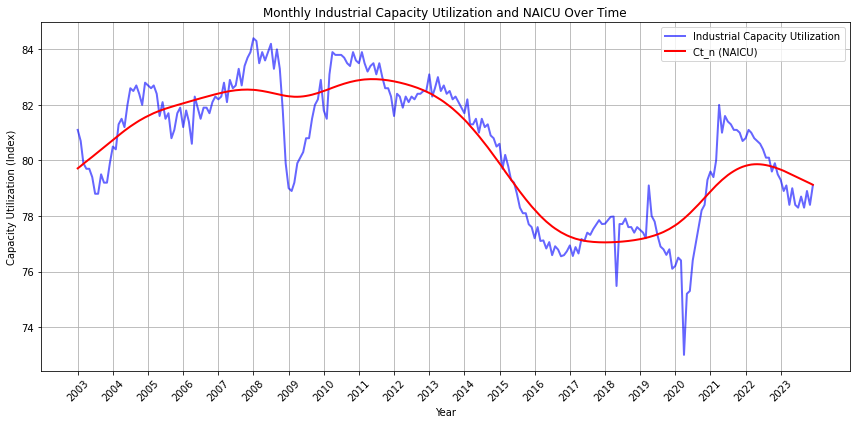
Figure 4: Monthly industrial capacity utilization and NAICU in Brazil from 2003 to 2023. Source: BCB and author’s calculations

The HP smoothing parameter, \(\lambda\), is suggested to be 1600 for quarterly and 100 for annual data. Since we have monthly data, we use \(\lambda = 14400\) as suggested by Hodrick and Prescott (1997).

Figure 5 shows the unemployment rate for Brazil from 2003 to 2023. The data is already provided in annual terms. We can see that unemployment was falling until 2014 – 2015 when it picked up again.

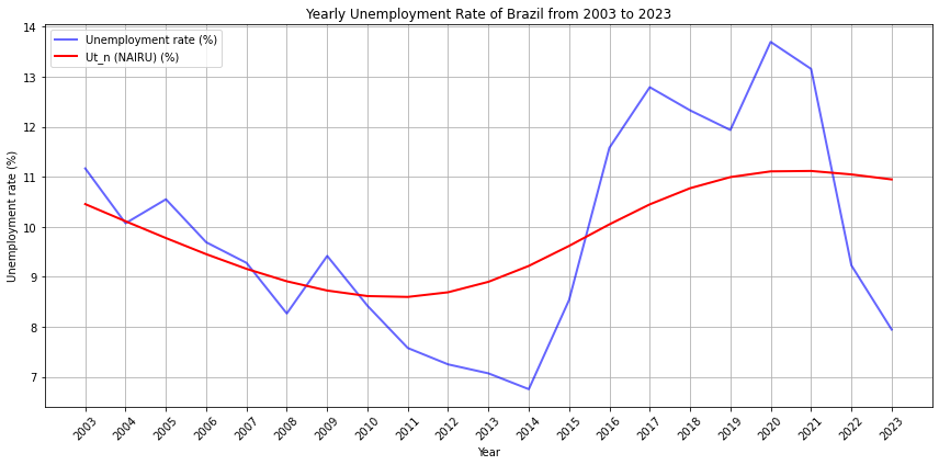
Figure 5: Yearly unemployment rate and NAIRU in Brazil from 2003 to 2023. Source: World Bank and author’s calculations

This is indicative of the 2014 – 2016 crisis that the Brazilian economy was going through. It started to fall until 2019 when it picked up again during COVID-19. For unemployment rate, a smoothing parameter value of \(\lambda = 100\) since the data is annual.

The capacity utilization and unemployment rate gaps are simply percentage deviations of the real value against the trend value. These gaps are shown in figures 6 and 7 respectively.

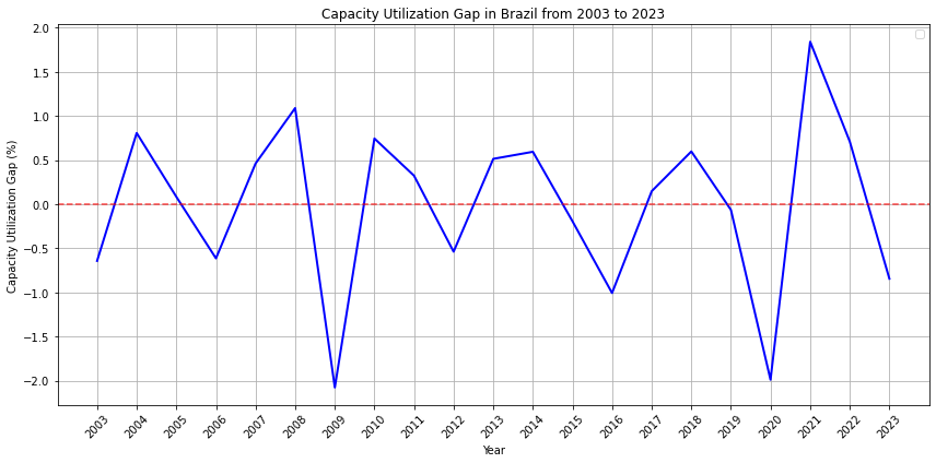
Figure 6: Capacity Utilization Gap (%) in Brazil from 2003 to 2023. Source: Author’s calculations

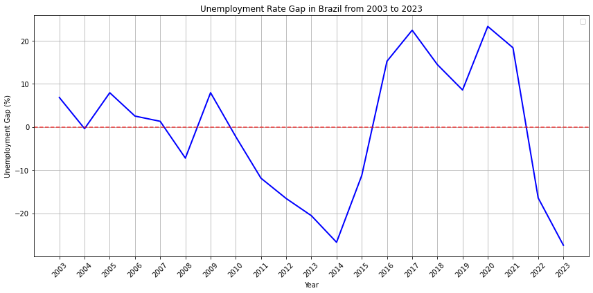
Figure 7: Unemployment Gap (%) in Brazil from 2003 to 2023. Source: Author’s calculations

We then simply use the equation to calculate the output gap:

Hence, we get the output gap as shown in figure 8.

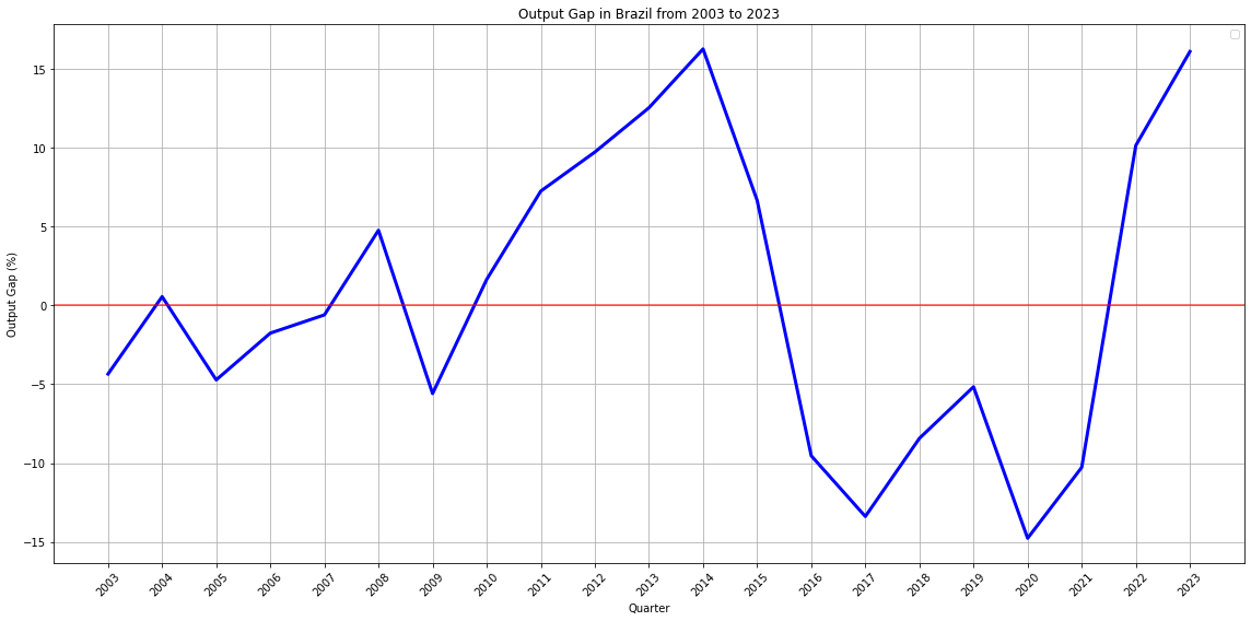
Figure 8: Output Gap (%) in Brazil from 2003 to 2023. Source: Author’s calculations

We can see the clear decrease in output gap during the 2015 – 2016 recession as well as the COVID-19 recession followed by the respective recoveries.

We now need to find the deviation from inflation. The inflation data is provided by the Extended National Consumer Price Index (IPCA). The target inflation rate is set by the National Monetary Council (CMN). A tolerance limit of ± 1.5% is followed to create a range within which inflation is tolerable. This is shown in figure 9.

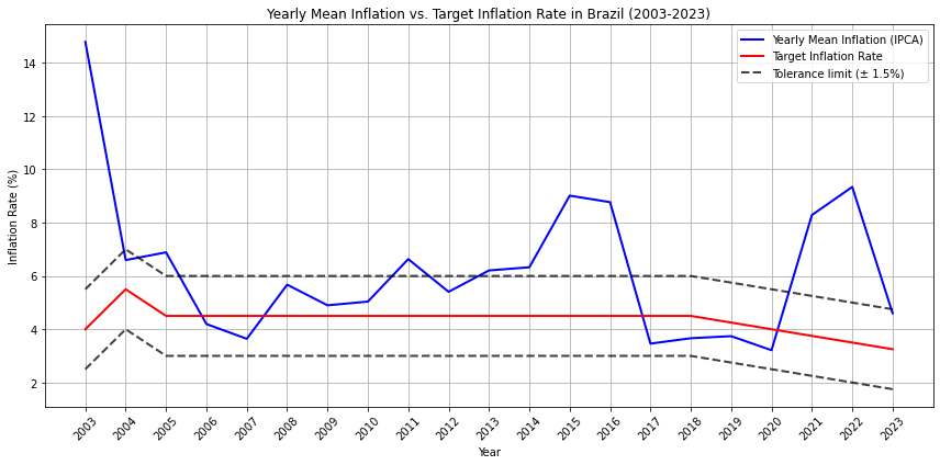
Figure 9: Yearly mean and target inflation rate in Brazil for 2003 to 2023. Source: BCB

From this, we can calculate the inflation gap by subtracting the target inflation rate from the IPCA inflation rate. This is shown in figure 10.

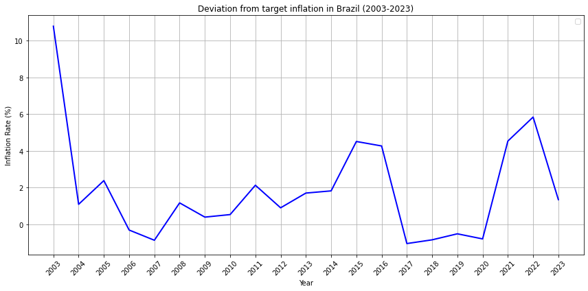
Figure 10: Deviation from target inflation in Brazil for 2003 to 2023. Source: Author’s calculations

This then gives us inflation as well as the deviation from inflation so now we can substitute the data into the Taylor Rule.

For the neutral real interest rate, we took it as 4.8% based on the BCB Inflation Report (June 2024).

We now have all the terms in the Taylor Rule equation to estimate the nominal interest rate.

Since Brazil has dealt with some tumultuous inflation in the past, the weight of deviation of inflation has been taken as \(a_\pi = 1.2\). This is to account for the heavy influence of hyperinflation and the central bank’s strict adherence to an inflation targeting framework. The weight of output gap has been taken as \(a_y = 0.5\). After calculating this through Python, we can plot the SELIC rate and the estimated nominal interest rate.

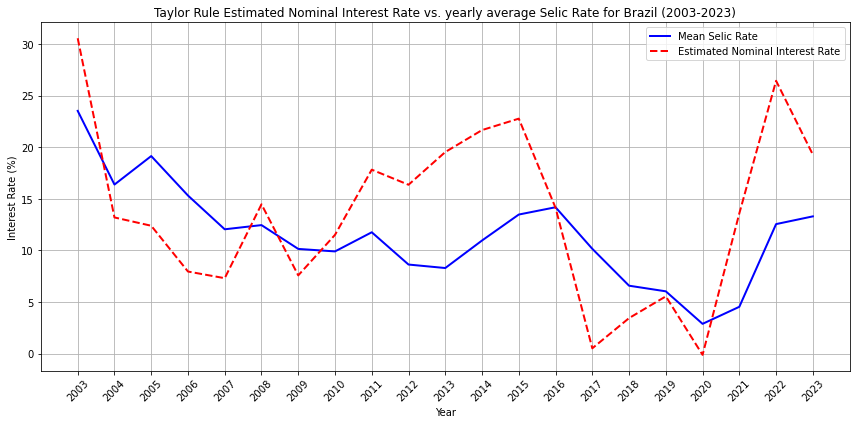
Figure 11: Average SELIC rate and the estimated nominal interest rate in Brazil from 2003 to 2023. Source: BCB and author’s calculations

We can see that there are various deviations and alignments that have happened between the average SELIC rate and the estimated nominal interest rate through the Taylor Rule. We can see that there were high spikes in the period of 2014 – 2016. This would have been due to the high period of growth that was occurring right before the economic crisis that led to a sharp decrease in GDP growth in 2016 and 2017. This is shown by the sharp drop in the estimated interest rate which almost reaches zero. The recovery period after the crisis again shows the Taylor Rule increasing in order to curb inflation. The estimated interest rate goes negative in 2020 which is as expected due to COVID-19. The increase in IPCA inflation, decrease in unemployment gap, and the increase in capacity utilization in 2021 due to the rapid recovery then shoots the estimated interest rate all the way to 15% before reaching about 28% in 2022. While the Taylor Rule was moved in various directions, the SELIC rate has not been as reactive. This is because, while the main goal is indeed inflation targeting, the central bank of Brazil (BCB) has focused a lot more on economic growth in recent times. This is evidenced twice in the periods 2011 to 2016 and then 2020 to 2022. The BCB has welcomed inflation by keeping the SELIC rate lower than the Taylor Rule.

While the Taylor Rule certainly provides a relevant benchmark for the nominal interest rate, it certainly is not used to justify or determine policy decisions. While the SELIC rate does indeed seem to follow the directions of the Taylor Rule at times, it certainly doesn’t match the rapid dynamics especially in terms of how high the interest rate should be.

Another aspect to consider is that this is still the basic Taylor Rule. Inflation-targeting frameworks usually incorporate a forward-looking mechanism in their discretionary rules. As such, we must modify the Taylor Rule in order to understand the BCB’s decisions.

Expectation-based Taylor Rule

We will modify the Taylor Rule to account for expected inflation instead of current inflation. The Taylor Rule will then be:

Where:

• \(E_t[\pi_{t+1}]\) is the expectation in the current period about the inflation of the next period

The yearly average of the expected inflation for the next 12 months is shown in the figure below.

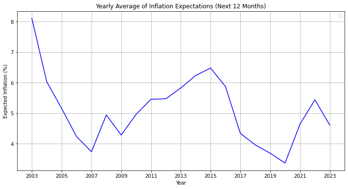
Figure 12: Yearly average of the expected inflation of next 12 months for Brazil (2003 to 2023). Source: BCB

After adjusting for expected inflation, the Taylor Rule estimated nominal interest rates changes as shown in figure 13.

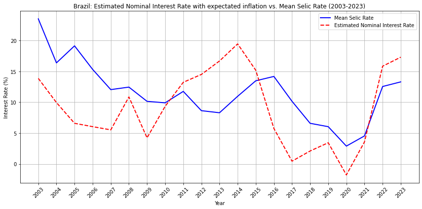
Figure 13: Average SELIC rate and the estimated nominal interest rate with expected inflation in Brazil from 2003 to 2023. Source: BCB and author’s calculations

We can again see that the Taylor Rule estimated nominal interest rate does suggest higher interest rates during high inflation periods as seen again during the 2011 – 2014 period. The sharp drop off from 2014 is also visible. In comparison to figure 11, where the Taylor Rule interest rate was based on current inflation, the expectation-based Taylor Rule fares better as it signalled a drop-off in interest rates in 2014 instead of 2015. As mentioned before, the BCB was more focused on growth and did not see the impending economic crisis at hand. As such, the SELIC rate ultimately followed the expectation-based Taylor Rule post 2016 though it was still higher than what the expectation-based Taylor Rule was suggesting.

We also again see the negative interest rate that is being suggested by the expectation-based Taylor Rule in 2020. It is suggesting an even lower negative interest rate than the basic Taylor Rule was suggesting.

What is most striking is the increase in the expectation-based Taylor Rule and the mean SELIC rate in 2021 where they increased in tandem for much of the start of the year before the continued increase of the expectation-based Taylor Rule towards the end. This shows that while the BCB does not alone follow the Taylor Rule, some aspects of the Taylor Rule are indeed embedded in the decision-making process of the BCB.

The expectation-based Taylor Rule then keeps on increasing in 2022 which is expected due to the expectation of high inflation from post-COVID-19 economic recovery. We can certainly conclude that not only does the expectation-backed Taylor Rule predict the dynamics of the Brazilian economy better, the SELIC rate also seems to move in tandem with it at times. In comparison to the basic Taylor Rule, the expectation-based Taylor Rule certainly is better.

Limitations of Taylor’s Rule

Although Taylor Rule has majorly benefited the monetary policy and its effectiveness, we see that there are quite a lot of challenges and limitations we face using Taylor’s in real life situations and scenarios. Here are few drawbacks of the same listed below:

1. There is quite oversimplification of economic dynamics which is assumed by this rule, one such is that it assumes that there might be a fixed relation between inflation, interest rates and output and does not take into account financial crisis, technological shifts or supply shocks.

2. This rule emphasizes on reliance on unobservable variables like potential GDP and natural rate of interest which in general are difficult to observe and their estimation might have quite a lot of uncertainty and the errors in estimating them might lead to less effective policy decision making.

3. There is quite inflexibility in this rule when it comes to crisis situations as the rule does not take into consideration certain economic risks like the asset bubbles or banking crises, complying to the rule in economic downturns or shocks could either lead to fairly tight or loose monetary policies.

4. The Taylor rule neglects exchange rate and other global factors that play a huge role in determining the country’s economic standing. The rule is quite domestically focused and does not take into consideration exchange rate fluctuations or global discrepancies. This is a major issue when estimating the Taylor Rule in Brazil. Considering that Brazil has been rocked by exchange rate volatility between the Brazilian Real and the American Dollar, adding in volatile variables that can affect the nominal interest rate is crucial. This is not mentioning the fact that Brazil is a commodity exporter and so the exchange rate is a crucial variable. Other such variables must also be identified and the Taylor Rule modified with these which can provide us with a much more accurate picture.

5. Another limitation is that the rule assumes one size fits all problems. The rule’s coefficients used for measuring inflation and output gap is quite outdated and might not fit all economies as they are not homogenous, rather they all need customized values based on their economic situations.

6. The rule cannot account for institutional challenges such as political pressure that prevent banks from complying strictly to the rule.

Conclusion

In conclusion, the Taylor Rule is an instrumental rule to determine the nominal interest rate. It identifies the key components that can affect the interest rate and formulates a mathematical model upon which the central banks can rely on. This has been evidenced by many central banks around the world that use the Taylor Rule as a discretionary rule.

However, it is not without its drawbacks. One drawback is that central banks must be forward-looking and as such, must use expected inflation. The basic equation of the Taylor Rule does not consider expected inflation but considering the time lags and minimal time to react to economic crises, expected inflation is a necessary variable. As shown in our analysis, expectation-based Taylor Rule certainly modelled the dynamics of the economy much better than the basic Taylor Rule.

Besides the basic and the expectation-based model, the Taylor Rule also leaves out crucial variables. In Brazil’s case, exchange rate is incredibly important due to the export orientation of the country. This leads to the question of what other variables are required to properly model the Taylor Rule in Brazil. Such answers will solve the drawbacks of the Taylor Rule which may propel it to an even more appreciated level within the monetary world.

Bibliography

1. Banco Central do Brasil (BCB). (2024, June). Output gap measures in Brazil. Banco Central do Brasil. Available at: Link

2. Banco Central Do Brasil (BCB). (n.d.). Time Series Management System. Available at: Link

3. Banco Central Do Brasil (BCB). (n.d.). Objectives and background. Banco Central do Brasil. Available at: Link

4. Banco Central Do Brasil (BCB). (n.d.). Banco central do Brasil. Banco Central do Brasil. Available at: Link

5. Bernanke, B. S. (2016, July 29). The Taylor rule: A benchmark for monetary policy? Brookings. Available at: Link

6. Blejer, M. I., Leone, A. M., Rabanal, P., & Schwartz, G. (2002). Inflation targeting in the context of IMF-supported adjustment programs. IMF Staff Papers, 49(3), 313-338. Available at: DOI

7. Brazilian Institute of Geography and Statistics (IBGE). (n.d.). Quarterly national accounts. IBGE | Portal do IBGE | IBGE. Available at: Link

8. Carvalho, F. G. (2022). The Central Bank of Brazil’s time-varying Taylor rule. Available at: Link

9. De-Losso, R. (2008). Did the Taylor rule stabilize inflation in Brazil? SSRN Electronic Journal. Available at: DOI

10. Hayes, A. (2003, November 24). Taylor rule definition. Investopedia. Available at: Link

11. Orphanides, A. (2003). Historical monetary policy analysis and the Taylor rule. Journal of Monetary Economics, 50(5), 983-1022. Available at: DOI

12. Sánchez-Fung, J. R. (2011). Estimating monetary policy reaction functions for emerging market economies: The case of Brazil. Economic Modelling, 28(4), 1730-1738. Available at: DOI

13. Twomey, B. (2010, January 3). The Taylor rule: An economic model for monetary policy. Investopedia. Available at: Link

14. World Bank. (2025, January). Unemployment, total (% of total labor force) (modeled ILO estimate) - Brazil. World Bank Open Data. Available at: Link

🔗 Repository

Source code and materials are available on GitHub:
👉 Taylor Rule Brazil Repository